


To govern is to foresee. For an IT department, everything starts with how resource consumption indicators evolve: storage, compute, bandwidth. A few days ahead, the job is to free up space or add capacity before something breaks. A few months or years ahead, it is to decide on investments. Mistral AI says Timestral, the time series forecasting model it released on 15 October, predicts these curves better than any competitor. We put it to the test on our own servers, against the methods IT teams have relied on for years. Let’s see how it does.
An AI that forecasts curves it has never seen
Time series forecasting did not wait for artificial intelligence. A time series is a metric recorded at regular intervals: disk space used, CPU load, website traffic. For decades, these series were extended with statistical methods, from linear regression to Holt-Winters exponential smoothing, developed in the late 1950s, and Box and Jenkins’ ARIMA models, published in 1970. Each applies a formula tuned series by series. From 2017, machine learning took over with tools such as Facebook’s Prophet and Amazon’s DeepAR, provided they were trained on the company’s own data and then maintained.
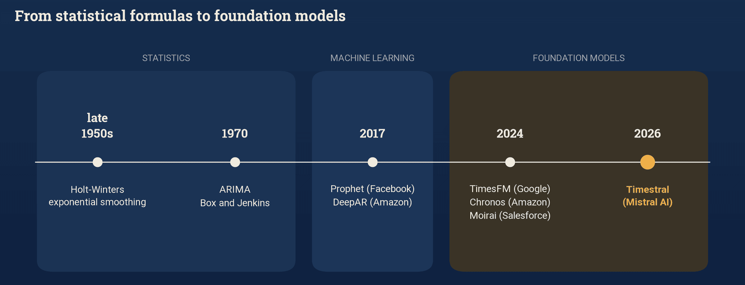
Since 2024, a third generation has upended this order. Google (TimesFM), Amazon (Chronos) and Salesforce (Moirai) took the architecture of large language models, the transformer, and trained it on billions of data points instead of text. These foundation models work zero-shot: they apply directly to a metric they have never seen, with no prior training.
Timestral is the latest arrival. According to Mistral, it beats its competitors on the field’s three reference benchmarks, and it “does not need a graphics card”. It comes in four sizes, from 5 to 209 million parameters. Its code is released under the Apache 2.0 licence and its weights are free for companies whose monthly revenue stays below 20 million dollars.
On paper, the promise is bold: a model that has never seen your servers would forecast their behaviour better than a formula tuned on them. We wanted to check that on ours.
The test: a month of forecasts, replayed
We extracted three months of hourly metrics from our own servers: storage space used, web traffic, number of requests received. We then ran a backtest, the standard way to evaluate a forecast. You go back to a date in the past, the model only sees the history up to that point, and you compare its forecast with what actually happened. We repeated this every day from 6 October to 2 November, 24 hours ahead, and every week since late September, seven days ahead. Since Timestral had never seen our data, the fact that these dates precede its release does not affect the result.
Three challengers faced it. Chronos-2, Amazon’s model, whose Apache 2.0 licence allows commercial use without conditions. Linear regression, which extends the trend of the last hours or days, and which Prometheus-family tools, VictoriaMetrics included, have offered for years as predict_linear. And the naive forecast, which simply repeats the previous day and serves as a yardstick.
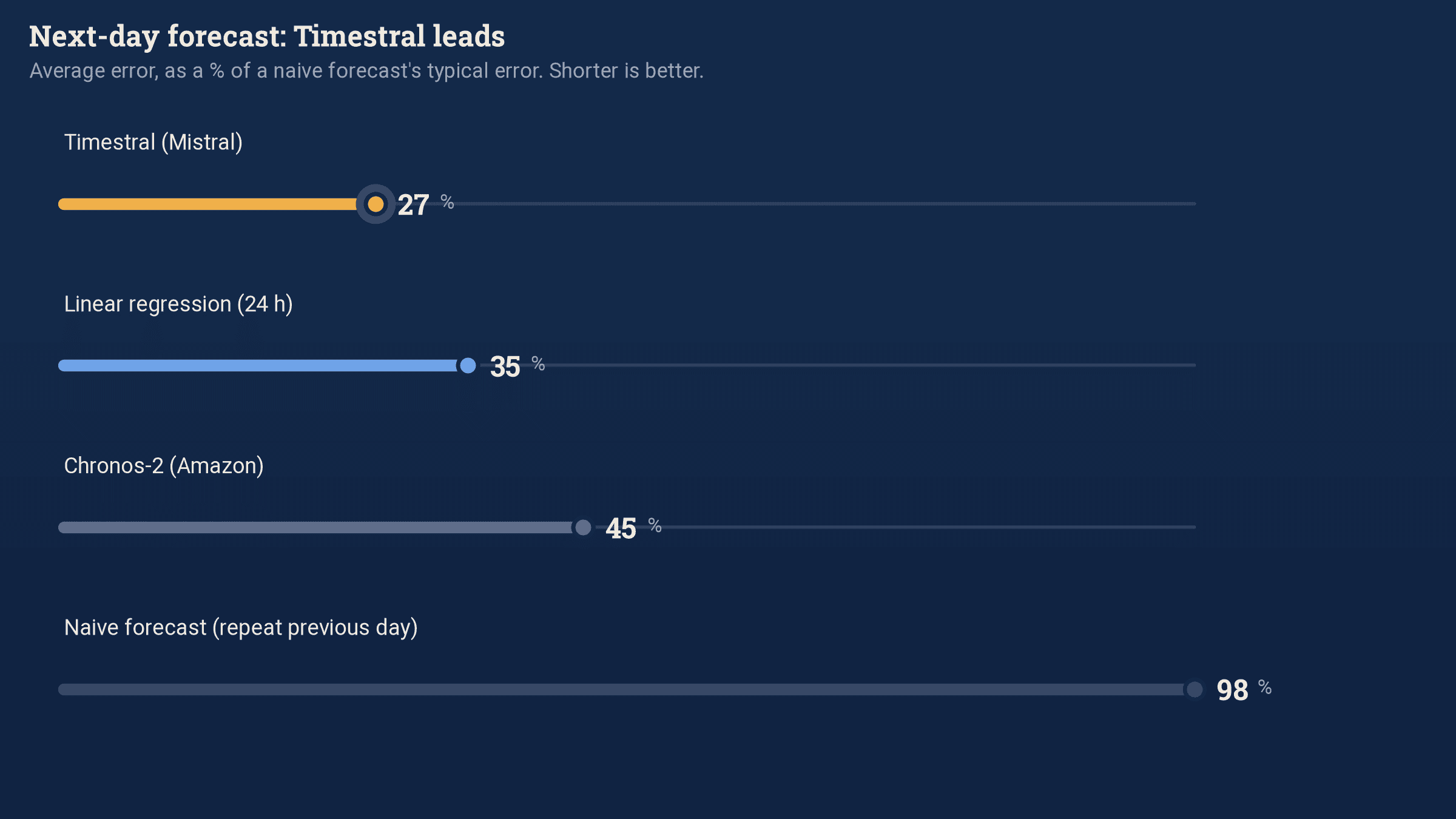
On next-day forecasts, Timestral delivers. Its average error is just over a quarter of the naive forecast’s. Linear regression does slightly worse, Chronos-2 clearly worse. Its 28-million-parameter version matches the largest one and produces each forecast in three hundredths of a second, on the processor of a Mac mini.
That left the question an IT department really cares about. Knowing the value of a metric tomorrow matters little in itself. What counts is the day it will hit a limit.
When will storage be full?
We asked the four methods that question, on the data volume of our two storage servers. On 21 occasions, we asked them when a threshold would be crossed, then measured the gap with the actual moment.
For a threshold reached the next day, all of them are off by a few hours. For a threshold reached a week later, the ranking flips. In median terms, the seven-day linear regression was off by 33 hours, Chronos-2 by 42 hours, Timestral by 45 hours. The oldest method beat the newest.
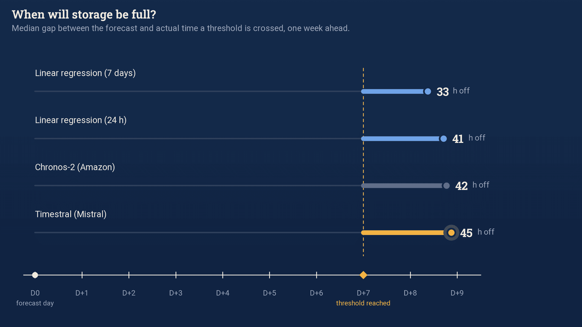
Timestral keeps one advantage: it always announces the crossing, whereas the regression computed on the last 24 hours alone missed it in 12% of cases. But every method announced the threshold too late.
To understand why they are all late, you need to look at one particular day.
28 October: 13,000 new series in one hour
That day, the number of series tracked by our infrastructure jumped by about 13,000 at once, and the volume stored on one of our servers rose by 400 megabytes in an hour. No method had foreseen it. None could have: nothing in the curve’s history announced it.
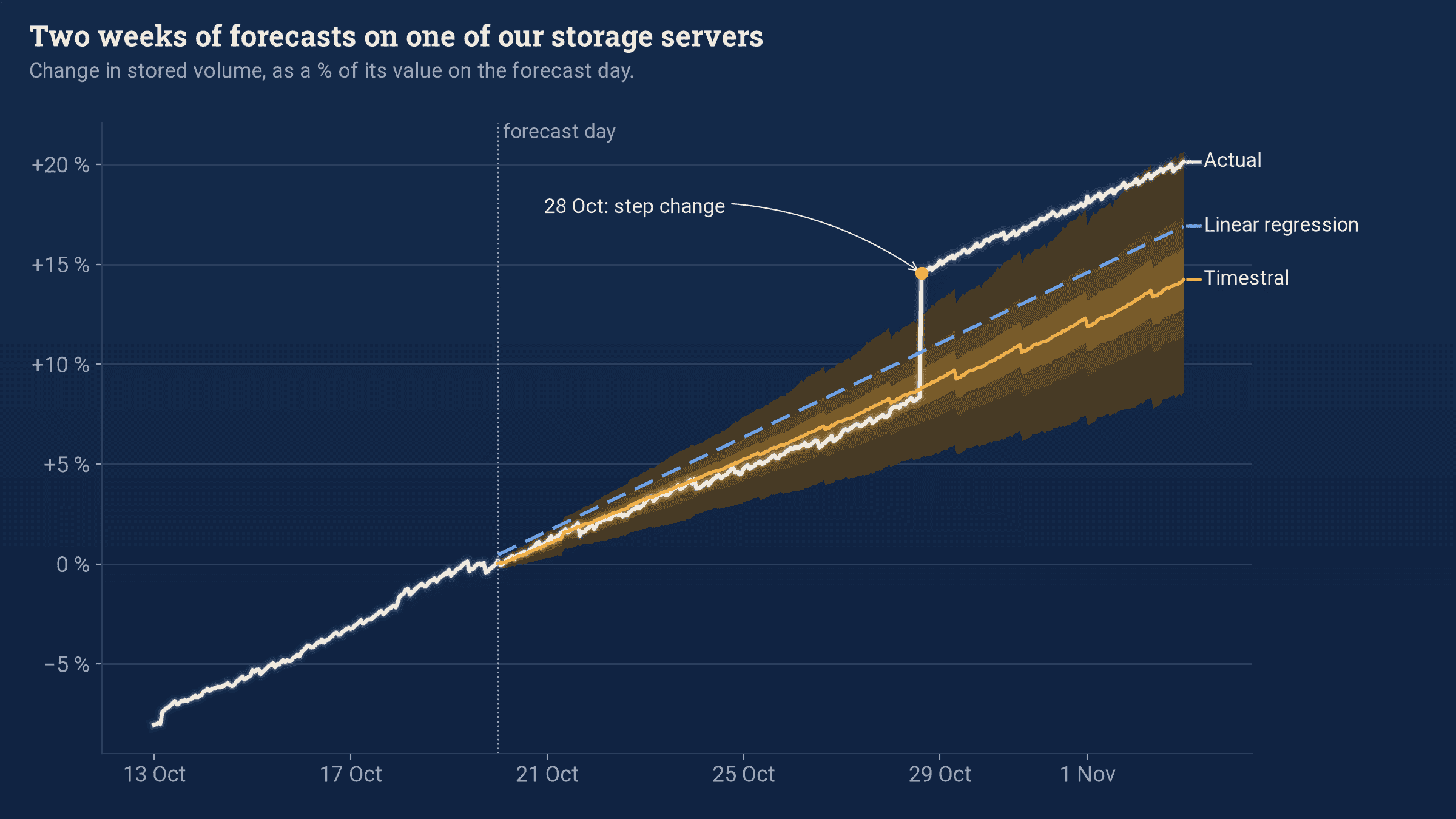
Every IT department knows this scenario. A new application goes live, a site opens, a migration moves users from one server to another: resource consumption jumps in a way nothing in its history announced. Curves do not rise smoothly, they climb in steps, and these steps account for most of the errors at seven days. A model cannot guess them. The teams preparing the go-live, however, often know about them weeks in advance.
Timestral can take that information in. Besides the history, it accepts known covariates, such as a production calendar or planned outages. We gave it the number of active series over the forecast period, as if the go-live calendar had been kept up to date. Its seven-day error fell by 8% on average, and by 15% on write throughput. On next-day forecasts, nothing changed.
The gain is modest, and we gave the model the actual figures, which no schedule can guarantee. It still shows where the room for improvement lies: in knowing what is coming, more than in the power of the model.
What we take away
Timestral is a good model, fast and cheap to run, but it does not replace existing methods. For monitoring storage saturation, linear regression remains a sound choice, and it is already available in VictoriaMetrics, the time series database we deploy for our clients. Models like Timestral find their place on metrics that follow a cycle, such as a website’s weekly traffic, and wherever a reliable forecast interval matters more than a single number.
Our test covers three months of history and the short term, from one to seven days. Planning investments several months ahead is a different exercise: it requires several years of history, with their budget and seasonal cycles.
The quality of a forecast depends first on what neither Mistral nor Amazon provides: metrics collected cleanly and without gaps, the choice of which series are worth forecasting, and an alert tuned to warn early enough without waking the on-call team for nothing. That is the work we do with our clients, with SenHub Agent for collection and VictoriaMetrics for storage, which we resell as a partner.
To govern is to foresee. On our servers, the best lead for forecasting better did not come from the newest model, but from the go-live calendar.
Key takeaways – To monitor storage saturation, the predict_linear function in Prometheus and VictoriaMetrics remains the right answer. One week ahead, it was off by 33 hours on our data, Timestral by 45. – For day-to-day forecasting of a metric, Timestral brings a real gain: an error almost a quarter lower than linear regression, computed on an ordinary processor. – Most errors come from steps, such as a new application going live, which no model can guess. Accuracy improves when the model is given the go-live calendar.
If you want to know what forecasting can bring to your own metrics, we can replay this backtest on your data. Contact us.
For technical teams
Information checked on 3 November 2026.
Data. Seven hourly resource consumption series from our infrastructure, from 3 August to 3 November 2026, with no gaps: storage space used on two servers, web requests, write throughput, read and write requests, and a raw counter reset twice during the test period.
Protocol. 28 daily origins at midnight UTC, 24 h horizon; 6 weekly origins, 168 h horizon; the full prior history is used as context, with no per-series tuning. Error measured as MASE (mean absolute error relative to the 24 h seasonal naive forecast, computed on the context), aggregated with a geometric mean.
Next-day results (MASE). Timestral-209M 0.27; Timestral-28M 0.27; 24 h regression 0.35; Chronos-2 0.45; 7-day regression 0.78; repeat previous day 0.98. Coverage of the 10%-90% interval: 79% for Timestral-28M, 80% for Chronos-2. At seven days, Timestral’s coverage drops to 63-67%: on our step-shaped series, its one-week intervals are too narrow.
Compute time. Median per forecast on a Mac mini M4, 8 threads, no GPU: Timestral-28M 0.03 s, Chronos-2 0.07 s, Timestral-209M 0.18 s.
Saturation. 21 daily origins, two nodes, thresholds set at the value actually reached 24 h, 72 h and 168 h later. Median gap at 168 h: 7-day regression 33 h, 24 h regression 41 h, Chronos-2 42 h, Timestral-28M 45 h. All methods are late.
Covariate. Number of active series provided as a known covariate over the horizon, actual values. Seven-day MASE from 1.58 to 1.45 on average, from 2.88 to 2.45 on write throughput. No effect at one day.
Limits. Seven series over three months, growing in steps. The results do not hold for every infrastructure. Chronos-2 and Timestral were used with their default settings. Licence: Timestral code under Apache 2.0, weights under a modified MIT licence, free below 20 million dollars of monthly revenue.
Sources. Mistral’s announcement; research paper; Chronos-2.


